Home Science Page Data Stream Momentum Directionals Root Beings The Experiment
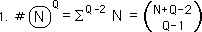
The potential impact graphs of the last Notebook, Time a Fractal Response, are based upon the following chain of reasoning. Below is a chart of the number of elements in the first few unravelings. Q represents the level of Unraveling. N is the number of Data Points in the Unraveling. The expression above the Q-numbers is the equation that was used. These were computed by brut force, using the equations 1->5 in a Study in Unraveling, Pages 1&2. The general equation is listed below the chart. This is not an easy equation to use, adding sums of sums of sums, depending upon the number of Unravelings. With a great number of Data Points the summations become prohibitive. We are looking for an expression that is not quite so difficult to compute.
What a surprise! Pascal's Triangle, diagonally across the chart. Note the circles. This is familiar territory.

Note also that the Q-values and N-values are symmetrical across the diagonal axis. This means that Q and N must be interchangeable in any general equation for the elements in an Unraveling. If either N or Q is increased in the same way, the number of elements increases identically. Q represents the number of Unravelings; N represents the number of Data Points. We've shown that increasing Q is like increasing the dimensionality of the construction of the Raveling numbers. Hence increasing N also increases the dimensionality of the structure. It could be said that this is a bi-multi-dimensional system because it has two interacting elements, Q & N, both of which increase the dimensionality of the structure.
Below is Pascal's Triangle in its normal orientation with the binomial expansion that is associated with it. The numbers in the triangle represent the coefficients of the expanded equation.

Below we place under each of Pascal's numbers, the N-value and Q-value from the Unraveling chart above (N left; Q right). Under the last row, when n=4, the combinations which determine the respective coefficients of the Binomial expansion are placed. These are well known expressions from the Binomial Theorem.

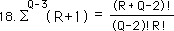
We've only looked at a finite number of samples for the number of elements in an Unraveling. We've seen a distinct pattern. We are going to take a logical leap, an extension of the pattern. This leap is verified experimentally and logically soon. But as of this writing this is no proof but only an extension of an apparent pattern. The assumption of patterns can lead to problems in the more complex manifestations, when the pattern subtly alters itself. In this situation, however, many factors combine to confirm the conclusions reached. We will leave the proof for more accomplished mathematicians. In extending the pattern we get the equation below, substituting the appropriate N's and Qs inside the combination symbol. Again this is a logical extension, not a proof.
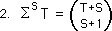
The general statement for the powers of summations of whole numbers is listed below. T is any positive integer. S is any integer from -1 on up, including 0. S replaces Q-2 and T replaces N in the general equation.
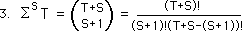
We extend the combination operation by definition.
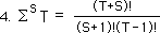
Combining terms we get this concise expression. This is the general expression for the multiple summations of integers.
Letting S take on different values, we see that it behaves as it is supposed to. Check the parallels with equations 1->5 in a Study in Unraveling, Pages 1&2. The T terms drop out when S = -1, leaving 1. This is the same as when Q is 1. There is only one element in the Unraveling.
When S = 0, only T is left. This equivalent to when Q is 2 and the number of elements is N.
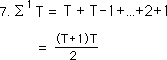
When S =1, we get the expression below, which is the common expression for the sum of consecutive numbers from one to T. This is what we hoped for.
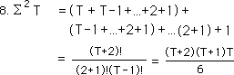
When S=2, equivalent to when Q =4, this is the expression we get, which corroborates our previous results. So not only does this combinatorial equation give us the same results as with other methods but it also yields this new expression for the double summation of positive integers.
Below is the general equation for Unraveling elements, (also derived from pattern analysis connected with experimental verification.) We plug in Q-2 for S and N for T in equation #4 immediately above.
This is the equation that falls out after combining terms. A second confirmation. Both N and Q have symmetric and interchangeable roles in the general expression. This was a necessary condition mentioned above.
Before we proceed let us discuss the internal symmetry of our diagrams. The Diagram on the left represents the fifteen elements of an Unraveling when Q=3 and N=5. The Diagram on the right illustrates how they are generated. It is the sum of a double unraveling of X5, a double unraveling of X4, and so on, to a double unraveling of X1.

Below is the Unraveling with all the elements in the same spots corresponding to the points in the diagram above.

It can be seen that each of the unique data points have been organized in rows, while the unravelings have been organized in columns. This horizontal organization is shown in the diagram on the left below. The diagram on the right shows the operations performed on each of the elements in the triple unraveling. Each of the elements in the vertical lines is divided by D, the Decay Factor. So the whole diagram is divided by D^2, once for each unraveling.

Each of the vertical and horizontal lines represents a scaling by K, which = (D-1)/D. Because of the internal symmetry in our diagram, each of the elements corresponding to a unique data point are scaled the same amount of times. Hence, although there are 15 elements to the unraveling, combing like terms we get only the five data points. See equation below.

Below left is the organization of the elements in general terms. The same principles that apply to the specific apply to the general. On the right is a scaling diagram. Each of the lines represents how many scalings, K, the data is from the Now. Now is defined as when R=0. R is the incremental time distance from the most recent Data Point. It turns out that each data point is scaled by its distance, in time increments, from the Now. When R=2, the potential impact of this Data point must be scaled twice, i.e. multiply by K, the scaling constant, twice, K2.

The internal structure of our geometric system is awesome. It is shown on the left organized by unravelings. In the middle we add the organization by data type. On the right we organize it as an equilateral triangle. It is organized from least scalings to most scalings by distance from the top.

The equilateral triangle has three lines of symmetry. Thus in determining the number of elements, what is true for one axis is true for all axes. Below is the three-dimensional geometry when Q=4 and N=5. With an additional Unraveling comes another dimension. Now we have an equilateral triangular prism, one of the divine regular solids of Greek geometry. At the pinnacle is the Now, R=0. Each of the Data Points is scaled from the top. With each additional Raveling comes another dimension. Thus when Q=5, we have a 4 dimensional equilateral triangular prism, a triangular prism within/without a triangular prism.
Remember from the above discussion that N and Q are interchangeable because of the internal symmetry of their interrelated geometry. This is true in terms of numbers of elements only, not in terms of scaling. Although the Data are only points while the Unravelings represents the number of extensional dimensions, geometrically they can be exchanged, because of the internal symmetry.
The dimensional representation of the number of elements in each Unraveling {See chart below with associated equation.} serves another purpose besides enumerating elements. It also serves as a scaling diagram. As one goes down on any of the prisms, the potential impact is scaled down. In algebraic terms, its potential impact is K times as great as the next higher level, where K, the Scaling Factor, equals (D-1)/D, where D is the Decay Factor. Also each triangular prism is also scaled down when moving right or Down. So each of these Dimensional Diagrams is also a Scaling Diagram. (And where there is scaling, there are fractals. And where there are fractals, there are also spirals. {See ahead for further edification.}) We had a two dimensional scaling diagram above. This is a 5 dimensional scaling diagram.

We find that each use of the data point is unique in terms of the scaling diagrams. The fifth point from the Now, i.e. R=5, has been scaled five times no matter the dimension. But the number of times it is used in each of the unique dimensions depends on how many different ways one can add up to five. If it is only one dimension, then there is only one way, 5+0=5. When there are two dimensions, there are 6 different ways of adding up 2 integers to 5: 5+0, 4+1, 3+2, 2+3, 1+4, and 0+5. When there are three dimensions, all the different possible routes are taken to reach 5 with 3 numbers. The basic point is that each element of each Raveling is unique. Although they are gathered together in large groups each one reached the same place from a different path. Also all the possible paths are used. No stone is left unturned but no stone is turned over more than once.
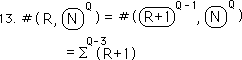
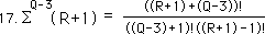
Let us return to the general expression for the number of elements in an Unraveling. Then let us expand the expression, once. This is what we get.
The first term indicates the number of terms in the reduced, Q-3, unraveling of XN. The last term of the equation represents the number of terms in the reduced unraveling of X1.
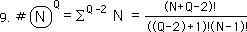
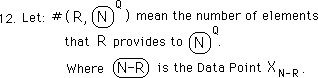
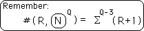
Let us now expand the # function, the number of elements function. Let the expression below represent the number of times that an individual data point appears in a multiple Unraveling. Check out the notational expansion.
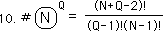
Now because of the internal symmetry principle mentioned above the elements of Data can be exchanged with the elements of Unraveling. The following equation is the result. Because each plane is symmetrical with the other triangular planes, no matter which dimension we travel on, the number of elements is interchangeable. The number of elements in the second horizontal plane of data from the top is the same as second vertical plane of Ravelings from the left. These equivalencies and their results find their algebraic expression below.
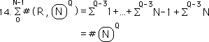
First expanding our equation from when R = 0 -> N-1, we get Equation #11, in reverse order, which is the total number of elements of Q Unravelings. This is what we were supposed to get.
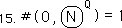
Employing Equation #13, when R = 0, leads to 1, the desired result. This is the Now, the pinnacle of our multi-dimensional triangular prism. It is only one point but is at the top of the pyramid.
Employing Equation #13, when R = 1, leads to Q-1, the desired result. This is the number of elements in the first data point after the Now. It is the number of elements in the first plane of data after the point at the top.
Extending and combining the results of equations 9 & 13, we get the following expression.
Combining like terms we get this equation to determine the number of elements in the Rth data plane below the peak, after the Now, when R=0.
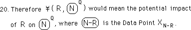
Before proceeding, we need to introduce more notation to deal with our mélange of ideas. Our topic is Potential Impact thus we introduce a potential impact notation.
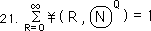
Before moving to any derivation, let us look at some necessary results. The first, and most essential, result is that the sum of all the potential impacts must equal one. This is a somewhat obvious result but bears examining. The value of any derivative number in any system is equal to the sum of the individual impacts that go into making it up. This is a truism and needs no further support.
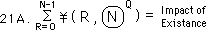
For Discontinuous Data Streams, with an unknown history or non-history, the equation below would be used for none of the points preceding the first Data Point are known. This is called the Impact of Existence. For Discontinuous Data Streams the Impact of Existence would equal the Total Impact.
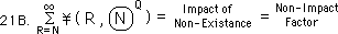
This is not enough for the derivatives of Continuous Data Streams because the impact precedes the first Data point. As mentioned earlier, a Continuous Data Stream starts from non-existence and then moves into existence. This differs from the Discontinuous Data Stream, which begins abruptly from an unknown prior history. So for Continuous Data Streams the period of non-existence contributes to the derivatives. Its potential impact diminishes with time but remains forever. This concept is expressed in the equation below. This equation is also a truism.
The potential impact of non-existence upon existence, non-being on being, nothing on something: henceforth when we speak of the Non-Impact Factor, this is what we are speaking about. The Non-Impact Factor pulls the measure down. The higher the Derivative the more the non-impact will pull it down. It is the disappearing part in the middle of the spiral squares. Its size depends upon D, the Decay Factor, N, the number of Data Points, and Q, the number of Ravelings, as we shall soon see.
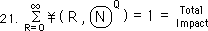
Thus when we add the Impact of Existence and Impact of Non-existence we obtain the Total Impact, for there is nothing left.
This is equation 21 above, the total impact, but remember this applies only to Continuous Data Streams. So one test of our equation would be to see if the infinite series for the different Unravelings would equal one, the total impact, 100%.
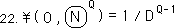
In the Notebook, Seed & Root Equation, it was shown that to unravel any number meant to divide by the Decay Factor, D, to the level of the diminished Unraveling, Q - 1. In the geometric examination above, it was shown that in determining the potential impact of each new dimension that all the elements of the Unraveling were divided by D, the Decay Factor. We've also seen that there is always only one element at the peak of our multidimensional pyramid. The impact of this peak element, the Now, when R=0, would have to be one, the number of elements, divided by D^(Q-1). Because it is Now, it is not scaled at all. Hence their are no K factors. The 'Q-1' represents the number of Unravelings or dimensions that the data is extended into.
Below is a dimensional Unraveling at the fourth level. The first Unraveling is the line of elements on the left, all to the 3rd power, divided by D. The 2nd Unraveling is the triangular plane of elements, to the right, all to the 2nd power, divided by D to the 2nd power. The 3rd Unraveling is a triangular pyramid of elements, on top and behind the front plane. Each element is divided by D to the 3rd power. Note that the D factor is applied each time there is a change in dimensions across the whole group of elements. The K factor, however, is nested behind parentheses. Hence each is element is scaled by K the number of times it is removed from the Now Data Point, XN.

Note that as the number of dimensions increases that the impact of the Now Data Point, XN, diminishes exponentially. In one dimension, Q=1, the impact is complete and immediate, no decay. To spread into 2 dimensions, however, decay is introduced. This diminishes the initial impact but then spreads it over time. Remember that no matter how impact is distributed, that the total always equals one. This law is the conservation of potential impact. It is a truism in a closed system, of which we are speaking. So the more dimensions that the data spreads into the more impact is spread over time and the less its impact is upon the Now derivatives. The impact of the data will still be 100% but will be spread over time. This is the phenomenon of Delayed Impact, which we spoke about in the discussion of the graphs.
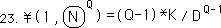
Remember that in systems of full and immediate impact, i.e., D = 1, that there is no decay and hence there is no separation. The first level of Decay extends immediately into all the dimensions that the Unraveling has. Hence the number of elements in first level of separation will be Q-1. Also it is only scaled once because it is only one level from the Now. But it still must be divided by D to the power of the number of dimensions, Q-1. This diminishes its immediate impact but conserves its impact so that it can spread through the dimensions. Below is the algebraic representation.
Remembering that number of elements on each individual plane is given by the equation below.
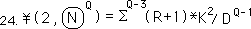
We apply this to the general impact expression. The number of elements in any dimensional plane is given by the above equation. The dimensional diminishment is given by the number of Unravelings, D^-(Q-1). At the second level of separation, when R=2, it is scaled twice because it is twice removed from the Now, XN. The algebraic expression is below.
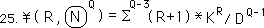
It is an easy step to a general expression for potential impact. If R represents the degree of separation from the Now, XN, and Q, represents the number of times that XN has been raveled then the equation below determines the potential impact of the data point upon the raveled measure in question.
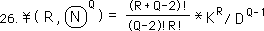
Applying the combinatorial equation, #18, we get this very usable equation.
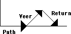
Below is a diagram that demonstrates each part of our equation. It is fairly self-explanatory. If you have any problems, ask your teacher.

Below is a diagram of the dimensions associated with the different levels of raveling. Notice that each dimension is built upon the scaled measures from the Dimension before.